
|
|
|
|
|
|
|
SimPolilla©
|
|||||||||||||||||||||||||||||||||||||||||||||||||||||||||||||||||
| Name of variable | Description | Parameter | Units |
|---|---|---|---|
| State variables | |||
| Elevation | Elevation on the study zone per cell i | Ei | meters above sea level |
| Temperature | Average temperature per cell i and month j | Ti,j | °C |
| Precipitation | Average amount of precipitation per cell i and month j | Li,j | mm |
| Habitat quality | Presence of potato cultures in cell i | Qi | Boolean |
| Higher-level variables | |||
| Moth abundance | Immature abundance in cell i | Ji | Number of individuals |
| Moth abundance | Adult abundance in cell i | Mi | Number of individuals |
| Moth abundance | Gravid female abundance in cell i | Gi | Number of individuals |
The higher-level entities are based on the number of insects of the three PTM species. Each time step represents one PTM generation based on T. solanivora life cycle duration (i.e. about 3 months at 15°C). An adjustment is made on the two other species so that each step corresponds to one PTM generation. The 500 per 500 m scale for cells was chosen for fitting the level of precision we have concerning PTM dispersion, based on available knowledge on moth dispersion (Cameron et al. 2002 [B]). Temperatures, precipitations and elevations have a 1 per 1 km resolution. Inside a square of four cells, these parameters have the same value.
In this section, we briefly describe the processes and scheduling of our model. Details are given in the submodels section. Each process is presented according to its sequence proceeding and in the order at which state variables are updated. Each time step is one T. solanivora generation.
Table 2. Processes of SimPolilla model
| Process | Submodel |
|---|---|
| State variable update | State variable update |
| Stochastic temperature | Stochastic temperature |
| Stochastic rainfall | Stochastic rainfall |
| PTM mortality | Crude mortality |
| Temperature dependent mortality | |
| Precipitation dependent mortality | |
| PTM dispersal | PTM neighborhood dispersal |
| PTM reproduction | Mating rate |
| Sex ratio | |
| Temperature dependent fecundity |
Each state variable corresponding to real data (Almanaque Electrónico de Ecuador by Alianza Jatun Sacha - CDC, digitised by DINAREN, 2003 ; Hijmans et al., 2005), is imported from individual files (one per layer), so that SimPolilla may be easily adapted to other regions.
Mean temperature is transformed according to a stochastic factor (Box & Muller 1958).
Three consecutive monthly precipitations are randomly chosen during a given step.
PTM population is updated according to crude, temperature and precipitation mortality.
PTM disperse through the territory from one cell to another by diffusion.
PTM populations are updated according to biological rules (mating rate, sex ratio, fecundity). A correction is made over fitness on the two other PTM species to adjust time step based on T. solanivora life cycle.
In Simpolilla model, moths' implicit objective is to infest the considered landscape by maximizing dispersal speed. Emergent key results are level of infestation in each cell and infestation speed. Interspecific interactions are not taken into account in this model and a stochastic factor over temperature and rainfalls are included mimic actual climatic variation.
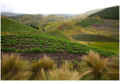
The environment is based on the Simiatug agricultural region (Bolivar, central part of Ecuadorian Andes), with temperature, precipitation and elevation from available data with a 1 km² resolution. The variables were obtained from the Worldclim data set (Hijmans et al. 2005) and the BINU Project (Biodiversity Indicators for National Use, Ministerio del Ambiente Ecuador and EcoCiencia 2005). Both temperature and precipitation data corresponded to the means of the period 1961-1990 (Hijmans et al. 2005). The cellular automaton is a 4-connex square shaped grid, with closed boundaries as we are considering an existing geographical location. At the beginning of each simulation, PTM inoculums are placed in the Simiatug village and spread is observed and recorded for each species.
In this section we describe the submodels given in table 2.
In order to feed the model with real climate variables, we chose to introduce a stochastic factor in the model (see also Sikder et al. 2006). We use the polar form of the Box-Muller transformation (Box and Muller 1958), to generate a Gaussian random number, based on climatic data from the region (see Dangles et al. 2008 - appendix A). Random number used is based on random procedure in VisualWoks (VisualWorks® NonCommercial, 7.5 of April 16, 2007. Copyright © 1999-2007 Cincom Systems, Inc. All Rights Reserved.).
As for temperature, we choose to introduce a stochastic factor to obtain a stochastic precipitation. Using a random number j from 1 to 12 (VisualWorks® NonCommercial, 7.5 of April 16, 2007. Copyright © 1999-2007 Cincom Systems, Inc. All Rights Reserved.), we use the monthly amounts of precipitation corresponding to three following months.
Data on development and survival for immature stages (eggs, larva, and pupa) and on fecundity for adults were acquired from two sources. First we used published data from laboratory experiments performed in the Andean region (Notz et al 1995; Dangles et al. 2008). Second we used data obtained within the last 8 years at the Entomology Laboratory at the PUCE (Pollet, Barragan and Padilla, unpublished data).
Overall force of mortality among a population is the sum of crude cause-specific forces. Here we consider dispersal related mortality (kd) and predation (ke) (see Roux, 1993; Roux et al, 1997) for P. operculella.
Sd,e(x) = e-(kd+ke)*x (1)
Temperature is the most basic controller in poikilothermic organisms (Zaslavski et al. 1988). Survival rate under laboratories conditions has been studied for the three PTM species, using a temperature dependent kinetic model (see figure 3 in Dangles et al., 2008).
Moth abundance was reduced by 80 %, when the cumulated rainfall during 3 consecutive months was higher than 600 mm (i.e. about 2.4 times more rainfall than on normal years).
The dispersal of the moths takes place during the adult stage when adults fly in order to find mates and/or suitable oviposition sites in potato fields (Barragán 2005). To include neighborhood dispersal into our model we considered the two factors:
These factors were integrated into our cellular automata for the three species, through:
VMi = 0.5 / { 1 + exp [ - (Mi - ß) / µ ] } (2)
where Mi is the number of adults in cell i, ß is the rate of increase in migration with density (transition center) and µ is the transition width. Due to the absence of data for potato moth about the parameters of the S-shaped curve, we fixed arbitrarily ß = 500 and µ = 75, i.e. we assumed a symmetric pattern of the curve from a moth density from 0 to half of K. A previous sensitivity analysis revealed that these two parameters had little influence on the overall dispersion of moths (Rebaudo and Dangles 2008).Pdist = exp-e*d (3)
where e is a fixed parameter of emigration rate (see below, Fig. 2). As stated by Cameron et al. (2002 [b]), little is known about the flight capacity of potato tuber moths, and the little information available is contradictory, with some reports suggesting limited flight capacity (Fenemore 1988, Palacios et al. 1997), and others indicating that adults are good fliers (Yathom 1968). These discrepancies can probably be understood by the fact that, as for many insects, flight capacities, especially at long distances, are closely related to wind conditions (Reed 1971, Goldson and Emberson 1977, Foot 1979). Cameron et al. (2002 [b]) measured a maximum dispersal distance of 250 m for P. operculella, a value that we used for T. solanivora and Symmetrischema tangolias, as we assumed that wind transport should be similar between the three species. Following Cameron et al. (2002 [b]), we fixed e to 0.015. Concerning dispersal at short distance, comparative observations of flight capabilities between P. operculella, Symmetrischema tangolias and T. solanivora in Ecuador revealed that the latter is a much worst flier than the former (Mesías and Dangles, pers. obs.) Although our model may overestimate moth neighborhood dispersal we preferred this to below estimation.Pcross(A,C,d) = { (A - (C-2*d)²) / A } with d[0:250] (4)
where A represents the cell's surface and C its length. Pcross was then multiplied by the probability of moths emigrating (eq. 3) in order to obtain the actual probability of moths leaving a cell, which we named Pleaving:Pleaving = Pcross * Pdist (5)
Finally, the number of moths dispersing to neighboring cells (Ndisp) was calculated as follows:Ndisp = VMi * Pleaving (6)
Fig. 3 shows effective dispersal rate in relation to moth density and flight distance. . Carrying capacity (K) was fixed to 1000 adults per cell i.")
Figure 1. Moth adults emigrating fraction as a function of adult density (eq.2). Carrying capacity (K) was fixed to 1000 adults per cell i.

Figure 2. Moth adults emigrating fraction as a function of distance as given by equation 3. Maximum flight distance was set to 250 m.

Figure 3. Effective dispersal rate considering moth density and flight distance.
Mating rate is correlated with age, sex ratio and weigh of individuals, but also with distance from one individual to another (Makee et al. 2001; Cameron 2004). No specific studies have been made on mating rate under natural conditions, and laboratory measurements may frequently represent an overestimation of the natural situation because laboratory females have little opportunity to avoid mating (Reinhardt 2007). However, as our cells are 500 m long, and thanks to field observation, we know that pheromones works at least on a 200 m radius, and we assume that within a cell, mating rate is equal to one no matter the density.
Among PTM population, sex ratio has been studied and is 1:1 (Saour 1999). After dispersal, the remaining adult population, combined with the mating rate and the sex ratio give the gravid females population.
Although energy-partitioning models have been developed to explain the shape of insect fecundity as a function of aging (Kindlmann et al. 2001), we are not aware of any mechanistic models that describes insect fecundity as a function of temperature. Several probabilistic non-linear models to fit insect fecundity across temperature have been proposed in the literature (Roux 1993; Lactin et al. 1995; Kim and Lee 2003; Bonato et al. 2007), but none of them gave us significant results with our data (r < 0.35, Fstat < 2.01). We therefore used weighted least square (WLS) regression to find the best model that fits our fecundity data across temperature. WLS regression is particularly efficient to handle regression situations in which the data points are of varying quality, i.e. the standard deviation of the random errors in the data may be not constant across all levels of the explanatory variables, which could be the case. For the three tuber moth species, the best fit was obtained with the Weibull distribution function, which has long been recognized as useful function to model insect development (Wagner et al. 1984).
The effect of temperature upon fecundity was well described by the Weibull distribution functions (r² = 0.75, 0.83, and 0.91 for T. solanivora, S. tangolias and P. operculella, respectively). Results showed marked differences among PTM species, both in terms of total numbers of eggs laid per females and optimal fecundity temperature : the highest fecundity was found in T. solanivora, with about 300 eggs/female at 19°C, followed by S. tangolias (220 eggs/female at 15°C) and P. operculella (140 eggs at 23°C).
Corresponding author : François Rebaudo
|
Centre de coopération internationale en recherche agronomique pour
le développement Informations légales © Copyright Cirad 2001-2015 cormas-webmaster@cirad.fr |
 OVERVIEW