
|
|
|
|
|
|
|
Wolf Sheep PredationPopulation dynamics between preys and predators
Version 1:In the first variation, the "sheep-wolves" version, wolves and sheep wander randomly around the landscape, while the wolves look for sheep to prey on. Each step costs the wolves energy, and they must eat sheep in order to replenish their energy - when they run out of energy they die. To allow the population to continue, each wolf or sheep has a fixed probability of reproducing at each time step. In this variation, we model the grass as "infinite" so that sheep always have enough to eat, and we don't explicitly model the eating or growing of grass. As such, sheep don't either gain or lose energy by eating or moving. This variation produces interesting population dynamics, but is ultimately unstable. This variation of the model is particularly well-suited to interacting species in a rich nutrient environment, such as two strains of bacteria in a petri dish (Gause, 1934).Version 2:The second variation, the "sheep-wolves-grass" version explictly models grass (green) in addition to wolves and sheep. The behavior of the wolves is identical to the first variation, however this time the sheep must eat grass in order to maintain their energy - when they run out of energy they die. Once grass is eaten it will only regrow after a fixed amount of time. This variation is more complex than the first, but it is generally stable. It is a closer match to the classic Lotka Volterra population oscillation models. The classic LV models though assume the populations can take on real values, but in small populations these models underestimate extinctions and agent-based models such as the ones here, provide more realistic results. (See Wilensky & Rand, 2015; chapter 4).The construction of this model is described in two papers by Wilensky & Reisman (1998; 2006) Description of the modelFrom the brief description above, but also from the analysis of the model code, we generated several UML diagrams.Here is the class diagram:  Class diagram of the model for version 2. Version 1"wolves and sheep wander randomly around the landscape, while the wolves look for sheep to prey on. Each step costs the wolves energy, and they must eat sheep in order to replenish their energy - when they run out of energy they die". Here is the translation into an activity diagram:
 Activity diagrams for the wolf and the sheep (version 1) Sequence diagram of version 1:  Results of version 1: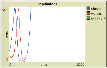
 As Wilensky explains, this version produces an unstable dynamic: either the extinction of the wolves and the demogaphic explosion of the sheep (because no grass limitation): left curves (in Netlogo), or extinction first of the sheep, followed by that of the wolves who have nothing to eat: right curves (in Cormas). Version 2The class diagram and the wolf activities remain identical. The activities of the sheep are now similar to those of the wolf:
Sequence diagram of version 2:  Results of version 2: incorrect replication
 Results of both implementations: left, original version under Netlogo, right, replication under Cormas. For version 2, we note a stabilization of the dynamics, which fluctuate but where the both populations are still presents. However, the results differ between the two platforms: in the original version under Netlogo (left graph), we note an average of 150 sheep and 75 wolves. In the version under Cormas (right graph), there are 200 sheep on average and less than 20 wolves. It was therefore necessary to understand where this important difference came from. Analysis of the different implementationsThe textual description of the model and its translation into class diagrams do not enable to get two convergent implementations. So we had to understand where this differences came from. After analysis of the Netlogo code, we understood that the difference came essentially from the random movement of the agents. In the case of Cormas, the predefined method of a random movement is called #randomWalk : it allows an agent to move from its cell to one of the 8 neighbouring cells taken at random. So it looks like a Brownian movement. In the case of the implementation of this model under Netlogo, the movement was written as follows: Here, each agent (turtle) moves one cell, but changing its direction by + or - 50°. This leads to a more oriented movement than a simple Brownsian movement. Yet this procedure, which was not described in the text, has important consequences on the overall dynamics of the system. This oriented movement has been re-implemented in the Cormas version. It was necessary to add an attribute called "direction" to the agents which, at initialization, contains a random value between 0° and 360°, as well as an attribute called "maxDeviation" valuing 50°. With these modifications, we obtain similar results:  In the same idea, we modified the original model under Netlogo to integrate the Brownian movement:  We then obtain dynamics similar to the 1st implementation under Cormas:  So here is the correct version of the class diagram that takes into account the oriented movements: 

|
|


